My First Deep Learning Project

Introduction

Over the past week I have been working on a Georgia Tech computer vision assignment [1] as a means of learning more about neural nets. The assignment was handed out by Dr. Derpanis for my colleagues and I to finish individually; he also turned it into a competition between us.

The assignment consisted of two parts. Both involved training a learning algorithm for a scene classification task. Part 1 consisted of training a neural network from scratch while Part 2 consisted of fine-tuning a pre-trained network (VGG-F) to fit the classification task.

There were 3000 images in total: 1500 training images and 1500 validation/test images. Validation and testing were treated as the same.

Accuracy is measured as 1 - lowest validation error.

Part 1

Before we get into improving the base neural net that was given, let’s take a look at it.

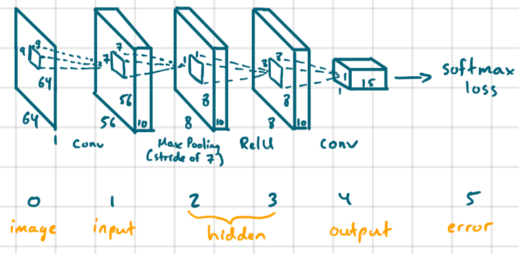
The issue with this network was that it was being overfitted to the training data with low accuracy (~27%). Let’s try to improve it.

Problem 1: We don’t have enough training data. Let’s “jitter”

As suggested in the assignment, we would need to jitter our training data in order to increase the amount of training data our net will see.

Before I did any of this, I changed my learning rate from 0.0001 to logspace(-4,-5.5,30) with 30 training epochs. This gave me a 3% accuracy boost. Then I upped it to logspace(-4,-5.5,100) with 100 epochs and I got another 2% accuracy boost. We’re at 32% accuracy.

I implemented simple image mirroring on all training data during the preprocessing step (in proj6_part1_setup_data.m). I avoided doing it in getBatch() (in proj6_part1.m) because I wanted to augment all of my training data instead of randomly choosing images in a batch and augmenting.

This gave me a 8.5% boost in accuracy. I tried randomly rotating and mirroring in getBatch() as suggested but that dropped accuracy by 3%. Not sure why. I guess it’s hard to beat having 3000 training images.

We’re at 41% accuracy.

Problem 2: The images aren’t zero-centered

As a means of normalization, I subtracted the mean image across all training and validation images from the training and validation set. This gave me a 14% accuracy increase. Oddly enough, computing the mean from only the training images (as suggested) gave slightly worse results.

We’re at 55% accuracy.

Problem 3: Our network isn’t regularized

Due to overfitting, we need to introduce a dropout regularization layer. This layer sets a certain percentage of inputs to zero for random neurons. It’s really effective but it also reduces the “learnability” of your network, as I have noticed. So use it carefully.

I inserted a dropout regularization layer before the final (fully-connected) convolutional layer with a rate of 50% and got a 7% accuracy increase.

We’re at 62% accuracy.

Problem 4: Our network isn’t deep

Before I started adding more layers, I decided to change the RelU non-linearity to a leaky RelU with a leak rate at 0.01. This gave me a 0.4% accuracy increase. I also changed the number of filters in the first convolutional filter from 10 to 20. This gave me a 1.4% accuracy increase.

Then I bumped it to 60 filters… 0.3% accuracy increase.

We’re at 64.1% accuracy. Getting close to the 66% reported by the professor who made the assignment!

Now it’s time to add more layers.

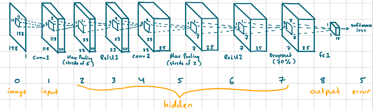
Basically, I increased the input resolution from 64x64 to 128x128; added a convolutional, max pool, and RelU layer; changed the dropout rate from 50% to 70%; and increased the number of epochs from 100 to 1000. All of this gave me a 1.5% accuracy increase.

We’re at 65.6%! Close enough! Ideally, I would have liked to hit 70% but that would have required more experimentation time.

Here’s how my final neural net for Part 1 looked like:

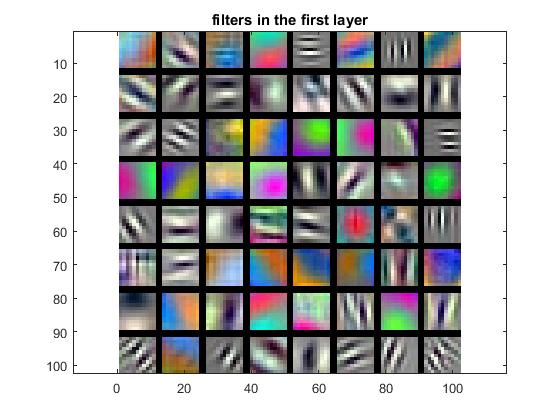
Here are the filters in the first layer:

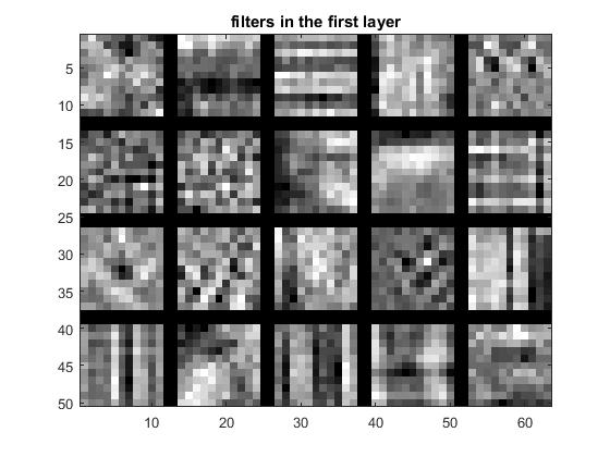
Note the horizontal/vertical edge filters and the gaussian-looking filter at [3,1].

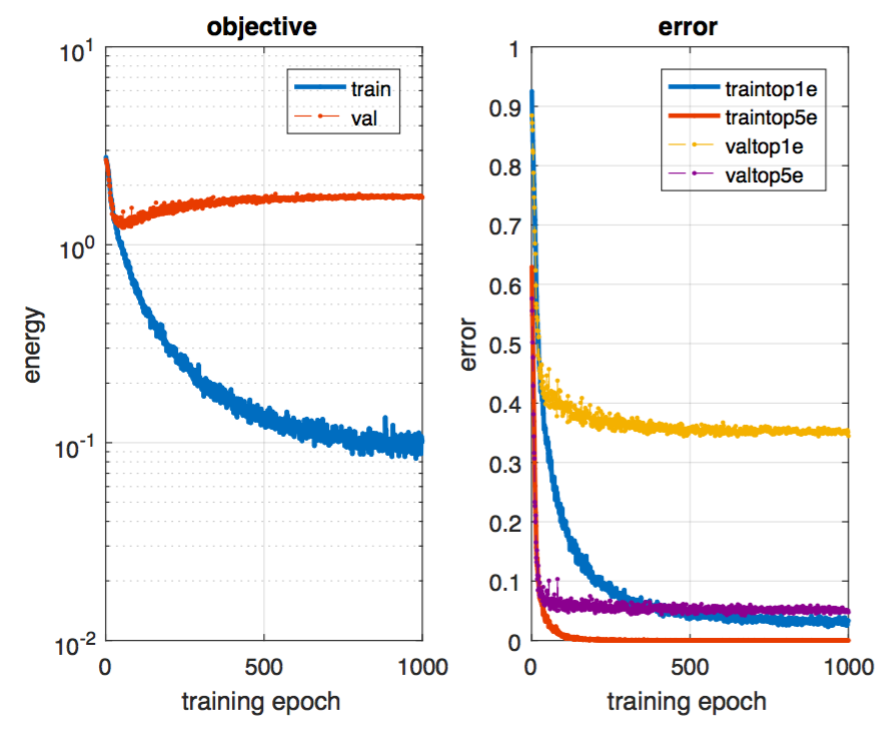
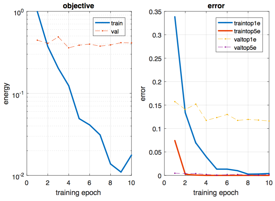
Here are the objective and error graphs over 1000 epochs:

Failed experiments

• Tried using colour filters but that didn’t work. Possibly due to the low filter resolution and depth.
  • Colour is very expressive and requires an expressive enough neural net (at least this is what I think).
• Data augmented with rotations and that made it worse.
  • Perhaps most of the test photos weren’t rotated by a non-negligible amount and I rotated test data too much.
• Used a deeper net with smaller filters.
  • Not enough training data, so it overfitted even with aggressive dropout.
• Initialized weights using a method discussed by He et al [2] which is meant for neurons with inputs coming from RelUs.
  • Not sure why this didn’t work out, I’ll have to look into it another time.
  • It caused divergence at an earlier rate and learning took way too long (even with a faster rate).
  • Supposed to be an improvement to the “Xavier” method of initialization [3].

If given more time…

• Implement Adagrad [4] for adaptive learning rates for each parameter.
  • Rare params get larger updates than frequently occurring params.
  • Could have fixed my experimentation issue with weight initialization using the He et al method.

• Try out “fancy PCA” (used in AlexNet in 2012) [5] for normalizing my data.

• Play around with different network configs and add more extensive data augmentation to fight overfitting.

Part 2

I implemented what was suggested by the professor. I added two dropout regularization layers (each with a rate of 50%) before fc7 and fc8; I used the same weight initialization method as I did in Part 1; I used the same jittering method as I did in Part 1; I kept the learning rate at 0.0001 and used 6 epochs of training time.

With these slight modifications, I was able to get 88.6% accuracy.

Here are the filters in the first layer:

Note that they are in colour because we modified our data setup to include colour images and we converted grayscale images into 3-channel grayscale images. These filters are a lot more definitive than the ones in Part 1. We can see edge filters in multiple orientations and in multiple colour combinations (including grayscale). We can also see some blobby structures as well.

Here are the objective and error graphs over 6 epochs:

Conclusions

I would have liked to have spend more time experimenting with Part 2 but I was held up on Part 1! I learned a lot about neural net architecture and how layers interact with each other. It was really useful being able to see the effects each type of layer had on the learning and testing process.

References

1. J. Hays. Project 6: Deep Learning. In Introduction to Computer Vision, Georgia Tech University, 2015.
2. K. He, X. Zhang, S. Ren, and J. Sun. Delving Deep into Rectifiers: Surpassing Human-Level Performance on ImageNet Classification. In ICCV, 2015.
3. A. Jones. An Explanation of Xavier Initialization. 2015.
4. R. Socher. Neural Tips and Tricks + Recurrent Neural Networks. In CS224d, Stanford University, 2016.
5. X.-S. Wei. Must Know Tips/Tricks in Deep Neural Networks . 2015.